- Research
- Open access
- Published:
Simultaneous optimization of even flow and land and timber value in forest planning: a continuous approach
Forest Ecosystems volume 8, Article number: 48 (2021)
Abstract
Background
Forest management planning involves deciding which silvicultural treatment should be applied to each stand and at what time to best meet the objectives established for the forest. For this, many mathematical formulations have been proposed, both within the linear and non-linear programming frameworks, in the latter case generally considering integer variables in a combinatorial manner. We present a novel approach for planning the management of forests comprising single-species, even-aged stands, using a continuous, multi-objective formulation (considering economic and even flow) which can be solved with gradient-type methods.
Results
The continuous formulation has proved robust in forest with different structures and different number of stands. The results obtained show a clear advantage of the gradient-type methods over heuristics to solve the problems, both in terms of computational time (efficiency) and in the solution obtained (effectiveness). Their improvement increases drastically with the dimension of the problem (number of stands).
Conclusions
It is advisable to rigorously analyze the mathematical properties of the objective functions involved in forest management planning models. The continuous bi-objective model proposed in this paper works with smooth enough functions and can be efficiently solved by using gradient-type techniques. The advantages of the new methodology are summarized as: it does not require to set management prescriptions in advance, it avoids the division of the planning horizon into periods, and it provides better solutions than the traditional combinatorial formulations. Additionally, the graphical display of trade-off information allows an a posteriori articulation of preferences in an intuitive way, therefore being a very interesting tool for the decision-making process in forest planning.
Background
A forest can be considered a set of stands, which are contiguous communities of trees sufficiently uniform in composition, age-class distribution and site quality, to distinguish each community from its adjacent ones (Helms 1998). In forest planning, decision-making processes often use optimisation approaches for developing optimal harvest schedules that will best meet the objectives of the landowners or land managers (Kaya et al. 2016). The main issue consists in determining when (and how) to harvest each stand during the planning horizon (next P years), to achieve the proposed objectives. To formulate this problem, it is necessary to have a simulator that allows predicting the development of forest stands efficiently and accurately. In the last decades, many papers have been devoted to this topic (see, for instance García 1994; Castedo-Dorado et al. 2007; Álvarez-González et al. 2010), and for any well-know species can be assumed that output functions are available, given, for example, the timber volume Vj(y) (volume/area) of the stand j along the time. To clearly show the novelty and interest of this work, we begin by analyzing different formulations of the forest planning problem in the optimization framework. For simplicity, we assume that maximizing timber volume is the main objective. Without any additional hypothesis, denoting Aj the area of stand j, the problem is to determine the harvest rate \(h^{r}_{j}(y)\) (area/time) of each stand over time (Heaps 1984; 2015), such that
Although this formulation is quite simple, the decision variable \(\mathbf {h^{r}}=(h^{r}_{j})_{j}\) is a vector function defined on [0,P], which makes the problem not easy to solve. For this reason, it was originally thought to assume that: (H1) interventions (cuts) on each stand j are instantaneous, at instants \(y^{k}_{j}\) set in advance (generally at the beginning, middle or end of the periods in which the planning horizon [0,P] is divided). Hypothesis H1 is equivalent to assume that \(h^{r}_{j}(y)=\sum _{k} A_{jk}\delta (y-y_{j}^{k})\), being Ajk the area of stand j cut at intervention k, and δ(y) the Dirac’s delta function (Oldham et al. 2009, Ch. 9). Under this hypothesis, problem (1) changes to find matrix A=(Ajk) such that
Taking the proportion of stand j cut at intervention k (xjk=Ajk/Aj) as the new decision variable, this problem is writing as
which is the so-called ‘Model I’ linear programming (LP) problem (Johnson and Scheurman 1977). It is widely used when the spatial location of the cutting areas must not be considered, can be exactly solved with the simplex method (Curtis 1962), and also with the reduced cost (RC) approach, which produces optimal, near-feasible solutions in a cheap and simple way (Hoganson and Rose 1984). If it is necessary to consider that location, an additional hypothesis must be assumed: (H2) the whole stand j can only be cut in a single instant yj (harvest instant). This hypothesis transforms the continuous variables xjk into binary variables (xjk=1 if and only if \(y_{j}=y_{j}^{k}\)), and (3) is changed into the combinatorial problem
Within the framework of the binary linear programming (BLP), the exact solution of (4) can be obtained by the branch and bound or cutting plane methods, as long as the problem does not exceed a certain relatively small dimension (Bettinger et al. 1999). For large problems, a spatial application of the RC method can be also useful (Pukkala et al. 2009). Additionally, problem (4) also accepts a combinatorial formulation in the frame of non-linear integer programming (NLIP), by considering the harvest instants \(\phantom {\dot {i}\!}\mathbf {y}=(y_{1},\ldots,y_{n_{s}})\) as the decision variables. In this case, (4) is equivalent to find vector y such that
This formulation is more appropriate if a heuristic method is used to solve the problem (which generates a solution within a reasonable amount of time, although of uncertain quality (Davis et al. 2001, p. 741; Bettinger et al. 2009, p. 172).
If hypothesis H1 is not considered, then H2 is equivalent to assume that \(h^{r}_{j}(y)=A_{j}\delta (y-y_{j})\), and without any additional assumption, problem (1) changes into the following non-linear problem (NLP)
Now, hypothesis H1 can be understanding as a discretization of the continuous variable of this NLP, and if it is assumed (what may be necessary if the dimension of the problem –number of stands–, is high and the available methods do not work in a reasonable time), problem (6) becomes straightly the previous NLIP problem (5). Equivalences and transformations between all these formulations are summarized in Fig. 1.

Equivalences and transformations between different formulations of the forest planning basic problem (harvest scheduling problem)
Problems (3)-(6) can be improved by considering more sophisticated goals, such as land and timber value (LTV). They can also be completed with additional objectives and/or constraints related to even flow of products (EF), size of contiguous area harvested (spatial constraints), etc. There are many papers dealing with models based on formulations (3)-(5), and Table 1 includes some examples classified by the formulation type, and the objectives and constraints considered. On the contrary, due to the inheritance of the original LP formulation, and to the apparent absence of suitable methods for numerical resolution, models based on the continuous formulation given in problem (6) have been much less explored (see, for instance, Roise 1990). The aim of this work is to help fill this gap in the forestry literature, by presenting a novel continuous bi-objective model in forest planning.
In recent papers, Arias-Rodil et al. (2017) and González-González et al. (2020) presented rigorous mathematical analysis of two continuous metrics for measuring, respectively, land expectation value (LEV) and EF. In this work, without losing their good properties for working with gradient-type methods, these metrics are appropriately modified to deal with the scheduling harvest problem of a forest, assuming future rotations based on economically optimal management prescriptions at stand level. These modifications include a novel way to estimate the planning horizon in an automatic manner, and the possibility that a stand is harvested several times. The combination of these new metrics leads to a bi-objective model, which can be efficiently solved by using gradient-type techniques, does not require to set management prescriptions in advance, and avoids the division of the planning horizon into periods, therefore resulting an useful tool for the decision-making processes in forest planning.
The paper is organized as follows. In Methods section, the new metrics are detailed in a suitable mathematical framework, and the forest planning problem is formulated by means of the new continuous bi-objective model, which is studied from a cooperative point of view, proposing a numerical method to obtain its Pareto-optimal frontier. The efficiency and accuracy of the numerical method is shown in Results and discussion section, where results in some Eucalyptus globulus Labill. forests are presented and discussed. Finally, some interesting conclusions are summarized in Conclusions section.
Methods
Mathematical framework
To formulate the forest planning problem, we need a growth simulator which allows prediction of stands development. To that end, we used the dynamic systems-based framework (frequently referred to as “state-space” approach), first used in forestry by García (1994). Particularly, our approach is based on:
-
Each stand j is characterized by three state variables: mean height of dominant trees in the stand(Hj, in meters), number of stems per hectare (Nj), and stand basal area (Gj, in m2/ha).
-
Outputs can be obtained from the predicted values of these state variables. For example, the timber volume (in m3/ha) is given by a known species-specific function vj(H,N,G).
We denote by ns the number of forest stands, and for each stand j we assume to know its age at inventory (\(t^{0}_{j}\), in years), area (Aj, in hectares) and measurements, at age \(t^{0}_{j}\), of the state variables (\(H^{0}_{j},N^{0}_{j}\) and \(G^{0}_{j}\)). In addition, we also assume to know species-specific transition functions hj,nj and gj given, from the previous data, the state variables at any age t≥0. That is, the state variables are given by \(H_{j}(t)=h_{j}(t^{0}_{j},H^{0}_{j},t),N_{j}(t)=n_{j}(t^{0}_{j},N^{0}_{j},t)\) and \(G_{j}(t)=g(t^{0}_{j},G^{0}_{j},t)\).
To avoid confusion, it is important to distinguish between stand age, denoted by t, and the time from the beginning of the planning horizon (inventory), which is denoted by y. Both are given in years, and if the age of a stand at inventory is t0, then y=t−t0. Particularly, if stand j is clearcut at time yj (when it is \(t_{j}=y_{j}+t_{j}^{0}\) years old), the timber volume is given by Vj(yj)=vj(H(tj),N(tj),G(tj)). The ultimate objective of forest planning is to determine the management prescription that will be applied to each stand. In this study, to alleviate notation, we seek only the times of clearcutting from the inventory, that is, the decision vector \(\mathbf {y}=(y_{1},\ldots,y_{n_{s}}) \in \mathbb {R}^{n_{s}}\). Obviously, finding y is equivalent to finding t=y+t0.
Economic metric: the land and timber value (LTV)
The economic value of the forest is the sum of the value of each stand j, which depends on:
-
The timber value at the first clearcutting, given by pjVj(yj), being pj the expected stumpage price.
-
The land expectation value (LEV), which accounts for all future rotations of timber that will be grown on the area after clearcutting the existing stand. The LEV is defined as the present value, per unit area, of the projected costs and revenues from an infinite series of identical even-aged forest rotations, starting initially from bare land (Bettinger et al. 2009, pp. 40-42). It only depends on the future rotation age, hereafter \(\bar t_{j}\), and is given by
$$J_{j}^{LEV}\left(\bar t_{j}\right)=\frac{\left(1+r\right)^{\bar t_{j}}\left(R_{j}(\bar t_{j})-C_{j}(\bar t_{j})\right)}{(1+r)^{\bar t_{j}}-1},$$where r∈(0,1] is the interest rate, and \(R_{j}(\bar t_{j})\) and \(C_{j}(\bar t_{j})\) represent, respectively, functions of present values of revenues and costs.
The land and timber value (LTV) can be defined as the present value of the sum of the timber value at the first clearcutting and the LEV just after clearcutting. For each stand j, it depends not only on the time of the first clearcutting (yj), but also on the future rotation age (\(\bar t_{j}\)). We only seek for yj and, consequently, \(\bar t_{j}\) has to be set in advance. We assume future rotations based on the optimal management prescription at stand level, in such a way that \(\bar t_{j}\) is the solution of the following optimization problem
Under this assumption, the LTV of the forest is given by
The regularity properties of JLTV are given by the properties of functions hj,nj,gj and vj, and we can assume that it is smooth enough (Arias-Rodil et al. 2017).
Even flow (EF) metric
Even flow (EF) and sustained yield are two of the oldest objectives of forest management. The first has been related to the concept of maintaining a stable timber supply (nowadays provisioning ecosystem services) through appropriate forest planning and management techniques. There are numerous examples of how to address the even flow issue in harvest scheduling. Some studies use constraints that ensure volume levels in each period within some upper and lower limits (O’Hara 1989; Murray and Church 1995) or that allow a certain variation in volume between periods (McDill et al. 2002; Constantino et al. 2008), while others include even flow as an objective in which volume variations between periods should be minimized (Kao and Brodie 1979; Brumelle et al. 1998; Ducheyne et al. 2004).
In this study we recover the concept of harvest rate (now volume/time) and seek for a constant rate during a period of T years, named tentative planning horizon for even-flow. It represents the period for which, clearcutting all stands at least once time, a stable timber supply is desired. The value of T is a technical decision, which depends on the species, site qualities, stand ages... of the forest.
We consider that interventions may not begin at the present time if, for example, the forest is too young. We denote by lj>0, in years, the minimum harvest age for each stand j, in such a way that tj≥lj should be verified. From these bounds, the instant a≥0 (years) when harvests can begin in the forest is given: it will be zero if any stand can be harvested now, otherwise it will be the minimum time guaranteeing tj≥lj. Specifically:
Then, a constant harvest rate is seek in the forest during the period [a,a+T], but harvest instants (yj) can be greater than a+T if it is good from an economic point of view. The admissible set of planning strategies is given by
where \(y^{*}_{j}\) is the best management prescription from an economic point of view, that is, the solution of problem
Taking into account that a management prescription can be greater than a+T, and assuming that all stands have to be harvested at least once during the planning horizon, its upper limit must be automatically computed by
We assume that the best EF corresponds with the following situation: all stands are harvested at least one time in the period [a,a+T], and the harvest rate for this period is constant. If we allow to cut each stand only once during the planning horizon [a,b(y)], the total harvested volume is \(\sum _{j=1}^{n_{s}}V_{j}(y_{j})\). However, we assume that future rotations will be based on the optimal rotation at stand-level, and consequently, it is possible that any stand must be cut more than once during the planning horizon. In this situation, the total harvested volume is
and the desired harvest rate is
where H(y) is the Heaviside function (Oldham et al. 2009, Ch. 9). Therefore, from the EF point of view, the objective is to achieve the next goal harvest rate function (see Fig. 2)

Example of harvest rate (top) and volume harvested (bottom). The grey solid lines represent real instant harvests (top, Eq. (10)) and real volumes harvested (bottom, Eq. (12)), while the black dashed lines represent goal harvest rate functions (top, Eq. (9)) and goal volume harvested functions (bottom, Eq. (11))
Assuming instant harvests, the real harvest rate must be written in terms of the Dirac delta δ(y). Specifically, it is given by (see Fig. 2)
The Dirac delta is not a function in the traditional sense, so the comparison between expressions (9) and (10) is not appropriate. Instead of comparing harvest rates we propose to compare the volumes harvested (goal and real), which are obtained by integrating those expressions (9) and (10):
The EF metric must measure the distance between both functions for the planning horizon [a,b(y)]. By using the associated distance to the L2 norm (Adams 1975), for any planning strategy y∈Yad, it is given by
where the minus sign is included precisely so that a higher value of JEF(y) corresponds to a greater similarity of the function V(y,.) to the goal function Vg(y,.), which is what is meant by a higher even flow.
Following (González-González et al. 2020), it can be proved that function JEF has continuous derivatives in almost all points, and an explicit expression for its gradient can be obtained.
Bi-objective model
In this work, it is assumed that the main goal of forest planning is to determine the management prescriptions to be applied to each stand (i.e., to determine y∈Yad) to get the best profitability (i.e., to maximize JLTV) with the highest possible even flow (i.e., to maximize JEF). Hence, the following Bi-objective Optimization Problem (BOP) is considered:
This problem must be studied from a cooperative point of view, looking for non-dominated admissible vectors, also known as efficient solutions or Pareto optima. An admissible vector y∈Yad is said dominated if there exists a better admissible vector, in the sense that it improves at least one objective, without making the other worse. If y∈Yad is non-dominated (Pareto optimum), the corresponding objective vector \(\mathbf {J}(\mathbf {y})\in \mathbb {R}^{2}\) is also known as Pareto-optimal, and the set of Pareto-optimal objective vectors is known as Pareto frontier (see Fig. 3). A more detailed definition can be seen, for instance, in Miettinen (1998, p. 11).

Example of an admissible set \(Y^{ad}\subset \mathbb {R}^{3}\) (corresponding with ns=3) and an image set \(\mathbf {J}(Y^{ad})\subset \mathbb {R}^{2}\), where the Pareto frontier is highlighted
As commented above, the final aim is to determine the management prescription to be applied to each stand. Therefore, a satisfactory solution must be chosen within the set of Pareto optima. A satisfactory solution is the best compromise for the preferences of the decision maker. These preferences may be articulated prior to the analysis (allowing to reformulate the BOP into a single objective problem through weights or/and treating some objectives as constraints), after graphing the Pareto frontier, or interactively in a progressive way (requiring to compute only some Pareto optima) (Miettinen 1998, pp. 61-65). In the next section we propose a numerical method for obtaining the set of Pareto optima and graphing the Pareto frontier. It allows to articulate preferences a posteriori, resulting in a very interesting tool for the decision-making process in forest planning.
Numerical resolution
The first step is to solve the single optimization problems (7), whose solutions are inputs for computing both metrics. The second step is to calculate the solutions of problems (8), which are necessary to determine the admissible set Yad. Functions \(J_{j}^{LEV}\) and \(J_{j}^{LTV}\) are smooth (they have the same regularity properties than functions h, n, g and v), and problems (7) and (8) can be solved by any gradient-type method. In this work, the L-BFGS-B algorithm (Nocedal and Wright 2006), implemented in the free and open-source Python library SciPy 1.0 (Virtanen et al. 2020), was used.
Regarding BOP (13), to take advantage of the regularity properties of JLTV and JEF, we propose to obtain the Pareto frontier by the weighting method (Miettinen 1998, pp. 78-84), solving each single-optimization problem by a gradient-type method, combined with a random multi-start if local minima are detected. It is also advisable to normalize the objective functions so that their objective values are of approximately the same magnitude. For the results presented in the next section, both objectives were normalized using the ideal objective vector (that obtained by maximizing each of the objective functions individually subject to the constraints of the problem) and an estimation of the nadir objective vector (given by the value of each objective function at the point where the other objective function reaches its maximum) (Miettinen 1998, pp. 15-19), weights were taking equally spaced, and the L-BFGS-B algorithm was used again without any multi-start procedure. To check this approach, BOP (13) was also solved by the evolutionary algorithm NSGA-II (Deb et al. 2002), widely used in multi-objective optimization, and already implemented in the Python library Inspyred 1.0 (Tonda 2020).
Results and discussion
We analyzed the usefulness of our approach in a real forest of Eucalyptus globulus Labill. located in the municipality of Xove (Galicia, NW Spain), considering a tentative planning horizon for even flow of T=13.5 years. The forest comprises ns=51 stands whose area and inventory data can be seen in Table 2. From these data, the state variables until clearcutting are computed from the specific transition functions given by (García-Villabrille 2015). Specifically:
-
\(H_{j}(t)=h\left (t_{j}^{0},H_{j}^{0},t\right)=\exp \left (X\left (t_{j}^{0},H_{j}^{0}\right)-\frac {\beta }{t^{\alpha }X\left (t_{j}^{0},H_{j}^{0}\right)}\right)\), where α=0.5989,
Table 2 Inventory data (columns 3-6) and hypothetical predicted data at one year after clearcutting (columns 7-10) for the forest of the case study. Aj: stand area in hectares, \(t_{j}^{0}\): stand age in years, \(H_{j}^{0}\): dominant height in meters, \(N_{j}^{0}\): number of trees per hectare, \(G_{j}^{0}\): stand basal area in m2/ha β=13.90, and
$$ X(a, b) = 0.5 a^{-\alpha} \left({a}^{\alpha} \text{ln}(b) + \sqrt{4 \beta{a}^{\alpha} + \left({a}^{\alpha} \text{ln}(b)\right)^{2}}\right). $$(14) -
\(N_{j}(t)=n\left (t_{j}^{0},N_{j}^{0},t\right)=\left (\left (N_{j}^{0}\right)^{-0.5}+1.995 \, 10^{-5}\left (\left (t\right)^{2}-\left (t^{0}_{j}\right)^{2}\right)\right)^{-2}\).
-
\(G_{j}(t)=g\left (t_{j}^{0},G_{j}^{0},t\right)=\exp \left (X\left (t_{j}^{0},G_{j}^{0}\right)-\frac {\beta }{t^{\alpha }X\left (t_{j}^{0},G_{j}^{0}\right)}\right)\), where α=0.9906,
β=21.16, and \(X\left (t_{j}^{0},G_{j}^{0}\right)\) is given by (14).
From these state variables, the timber volume (m3/ha) is given by
After clearcutting, we assume no changes on site quality (site index) and a constant plantation density of 1333 trees/ha for all stands. Under this hypotheses, by using an appropriate function for initializing the stand basal area (García-Villabrille 2015), we predicted the data at one year after clearcutting (see Table 2). These data were used for computing the state variables (and outcomes) after the first clearcutting. To further test our approach in a forest with a different structure, we also used these data for simulating a hypothetical forest (hereinafter the simulated young forest) with 51 stands of the same species, area and site index, but all at one-year age.
For the real forest of the case study, Fig. 4 shows the Pareto fronts obtained with the weighting method and with the NSGA-II, for a population size of P=200 individuals and G=500 generations. Additionally, this figure also shows the comparison between real and goal volumes corresponding to all (ten) Pareto optima obtained with the weighting method. The corresponding results for the simulated young forest can be seen in Fig. 5. In view of these results, it can be highlighted that:
-
Both methods, although using different techniques, provide the same Pareto fronts, which warrants the appropriateness of our approach.
Fig. 4 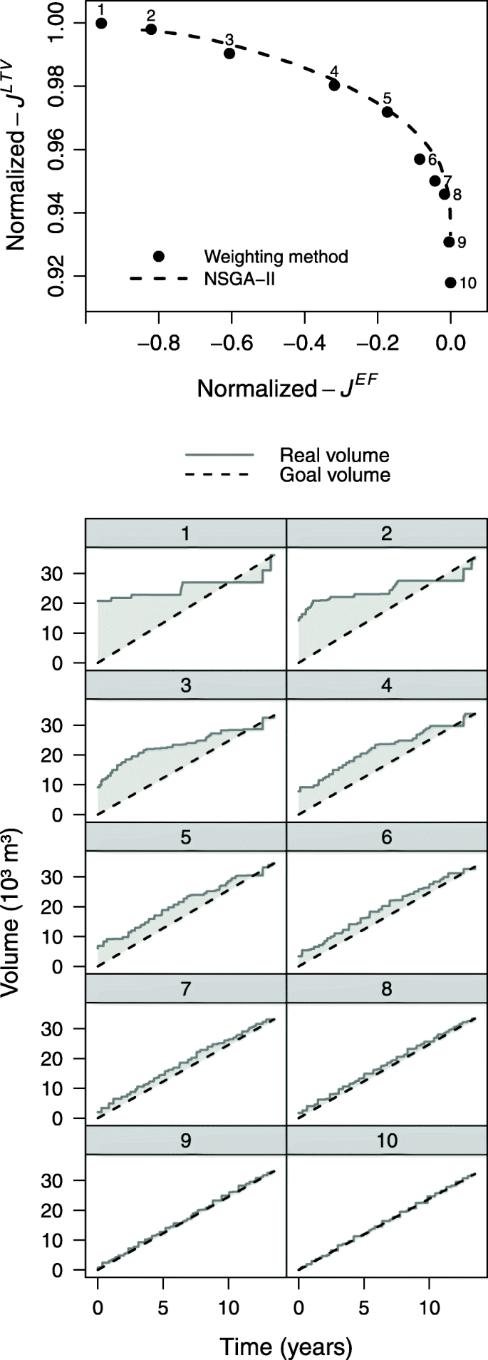
Results for the real forest: normalized Pareto front obtained with the weighting method and the NSGA-II (top), and comparison between real and goal volumes for the points obtained with the weighting method (bottom)
Fig. 5 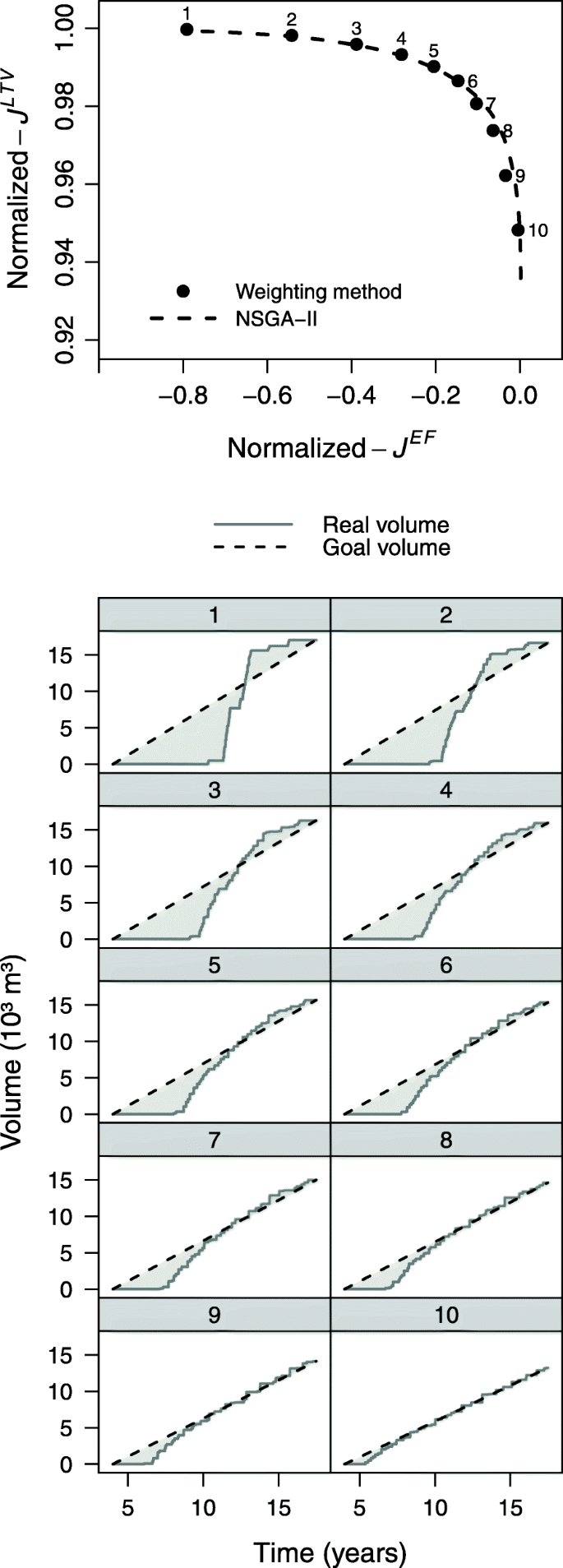
Results for the simulated young forest: normalized Pareto front obtained with the weighting method and the NSGA-II (top), and comparison between real and goal volumes for the points obtained with the weighting method (bottom)
-
The continuous approach works well for forest with very different stand structures, as suggested from the results of the real forest (which has many mature stands of different ages) and the simulated young forest (in which all stands are of the same age).
-
Figures 4 and 5 are very useful for the decision-making process:
-
In the top graphs, the normalized- JLTV is JLTV/JLTV(y∗), i. e., the LTV divided by its best value. This way of proceeding allows an intuitive comparison of the different optimal management strategies: for the real forest, there was a reduction of about 8% in LTV between the best solutions from the economic and even flow perspectives (points 1 and 10 in the Pareto front, respectively), while for the simulated young forest it was of only 5%.
-
The even flow metric has not such an easy interpretation in terms of numerical values, but the grey area of the bottom graphs of the figures clearly indicates the achievement of the even flow objective as well as the moment in which the clearcuts are done. Additionally, these graphs also show the total harvest volume of each Pareto optimum, which is reduced as the even flow objective is improved.
-


Finally, to analyze our continuous approach in larger forests, we simulated two new hypothetical forests: one with 204 stands and other with 1632 stands. They were obtained by replicating the stands of the real forest 4 and 32 times, respectively, and randomly generating their area between the minimum and maximum real-area values. Then, we solved the problem on the simulated forest with 204 stands and observed that the weighting method captured the complete Pareto front in a very reasonable time (about half a minute), but the NSGA-II needed a greater number of generations than the previous experiments with the 51-stand forests and, consequently, a higher computation time. This fact was confirmed by the results obtained on the simulated forest with 1632 stands, where the weighting method kept providing the complete Pareto front in an acceptable time (about seven minutes), but the NSGA-II with G=2000 generations only captured a small arc (see Fig. 6), with a computation time of about eleven hours. Table 3 summarizes the computation time of all performed experiments.

Normalized Pareto fronts obtained with the weighting method (∙) and the NSGA-II, for two simulated forest comprising 204 stands (top) and 1632 stands (bottom). The Pareto fronts obtained with NSGA-II correspond with a population size of P=200 individuals and a number of generations of G=500 (dashed line) and G=2000 (solid lines)
The use of non-linear continuous models to formulate the forest management problems has been scarce. In the framework of optimal control theory, Heaps (1984; 2015) studied the general problem of determining the harvest rate of each stand over time, but did not address with examples how the continuous forestry age class model he proposed could be solved numerically. Tahvonen (2004) discussed the use of discrete or continuous variables in describing time and age class structure in models for optimization of forest harvesting. Roise (1990) proposed and solved a continuous model, but without performing a mathematical analysis of the objective and constraint functions, applying optimization techniques that may not be the most adequate to solve the problem. On the contrary, the continuous model proposed in this paper uses functions with appropriate regularity properties, that guarantee a successful numerical resolution using gradient-type methods.
In this study we have dealt with a species whose main use is pulp production, therefore the land and timber value has been calculated on the basis of the stumpage price times the volume at the harvest instant. Nevertheless, for other species which require merchantable volume estimates, a more sophisticated method must be used. For example, in a study of optimization at stand level, Arias-Rodil et al. (2015) evaluated two alternative methods of estimating the merchantable volume of a stand at a given age: (i) a disaggregation system, which involves aggregating the merchantable volume previously predicted by diameter classes, and (ii) a stand volume ration function. The latter considers a top diameter limit for classifying the volume by timber assortments, while the former also allows specification of long length requirements. The use of alternative (i) may cause discontinuities in the JLTV function, which makes a gradient-based search challenging. However, alternative (ii) does not present any problem and, although will provide slightly higher optimal values of JLTV, may even be more accurate (Arias-Rodil et al. 2016).
Our proposal provides a graphical tool to analyze the relationship (trade-off) between the two objectives, helping the landowners to choose a suitable weighting after seeing the effect of even-flow requirement on economic profitability. This methodology can include constraints and be extended to other objectives, in pairwise comparison or considering three or more objectives. In the latter case, despite a posteriori techniques combined with special visualization methods have been used in forest management problems (Borges et al. 2014), interactive techniques can also be useful (Diaz-Balteiro 1998). In any case, the features of the problem and the capabilities and type of the decision maker have to be considered before selecting the most appropriate solution method (Miettinen 1998, pp. 227-231).
Conclusions
In this paper we present a novel continuous bi-objective model (economic vs. even flow) in forest planning. According to the results obtained, it is worth highlighting the following aspects:
-
The planning horizon is not set in advance and only a tentative value is required. It is involved in the optimization process and obtained as an output of the model.
-
The LTV and EF functions have smooth enough properties, which allows the use of gradient-type methods for its optimization, behaving in a more efficient, effective and robust way than many other gradient-free methods commonly applied in forestry.
-
The continuous formulation does not require to set management prescriptions in advance and avoids the division of the planning horizon into periods, providing solutions which may be better than those obtained with traditional combinatorial formulations.
-
This model allows forest-level problems to be treated with continuous decision variables, in a way similar to that used generally with stand-level problems. As envisaged in previous works, the performance of the continuous approach combined with gradient-type methods improved as the forest size (the number of decision variables) increased.
-
With this approach, it is not necessary to articulate the preferences of the decision maker a priori. Furthermore, the graphical outputs of our numerical method provide the Pareto front and other useful trade-off information in an intuitive way, which makes the proposed continuous bi-objective model a very interesting tool for the decision-making process in forest planning.
-
This model was successfully used in forests comprising single-species, even-aged stands which are intended to be managed with the rotation forest management system. The applicability of the model in forests with more complex structures and dynamics (forests consisting of mixed stands, which have gradual advance regeneration, and are treated with partial cuttings) is the topic of an ongoing research.
Availability of data and materials
All data generated or analyzed during this study are included in this published article.
Abbreviations
- BLP:
-
Binary linear programming
- BOP:
-
Bi-objective optimization problem
- EF:
-
Even flow
- LEV:
-
Land expectation value
- LP:
-
Linear programming
- LTV:
-
Land and timber value
- NLIP:
-
Non-linear integer programming
- NLP:
-
Non-linear problem
- NW:
-
North West
References
Adams, RA (1975) Sobolev Spaces. Academic Press, London.
Álvarez-González, JG, Zingg A, von Gadow K (2010) Estimating growth in beech forests: a study based on long term experiments in Switzerland. Ann For Sci 67(3):307.
Arias-Rodil, M, Barrio-Anta M, Diéguez-Aranda U (2016) Developing a dynamic growth model for maritime pine in Asturias (NW Spain): comparison with nearby regions. Ann For Sci 73(2):297–320.
Arias-Rodil, M, Diéguez-Aranda U, Vázquez-Méndez ME (2017) A differentiable optimization model for the management of single-species, even-aged stands. Can J For Res 47(4):506–514.
Arias-Rodil, M, Pukkala T, González-González JM, Barrio-Anta M, Diéguez-Aranda U (2015) Use of depth-first search and direct search methods to optimize even-aged stand management: a case study involving maritime pine in Asturias (NW Spain). Can J For Res 45(10):1269–1279.
Baskent, EZ, Keles S, Yolasigmaz HA (2008) Comparing multipurpose forest management with timber management, incorporating timber, carbon and oxygen values: A case study. Scand J For Res 23(2):105–120.
Bettinger, P, Boston K, Sessions J (1999) Intensifying a heuristic forest harvest scheduling search procedure with 2-opt decision choices. Can J For Res 29(11):1784–1792.
Bettinger, P, Sessions J, Boston K (1997) Using Tabu search to schedule timber harvests subject to spatial wildlife goals for big game. Ecol Model 94:111–123.
Bettinger, P, Graetz D, Boston K, Sessions J, Chung W (2002) Eight Heuristic Planning Techniques Applied to Three Increasingly Diffi cult Wildlife Planning Problems. Silva Fennica 36(2000):561–584.
Bettinger, P, Boston K, Siry JP, Grebner DL (2009) Forest Management and Planning. Elsevier, Amsterdam.
Borges, JG, Garcia-Gonzalo J, Bushenkov V, McDill ME, Marques S, Oliveira MM (2014) Addressing multicriteria forest management with Pareto frontier methods: an application in Portugal. For Sci 60(1):63–72.
Boston, K, Bettinger P (1999) An analysis of Monte Carlo integer programming, simulated annealing, and tabu search heuristics for solving spatial harvest scheduling problems. For Sci 45(2):292–301.
Brumelle, S, Granot D, Halme M, Vertinsky I (1998) A tabu search algorithm for finding good forest harvest schedules satisfying green-up constraints. Eur J Oper Res 106(2-3):408–424.
Castedo-Dorado, F, Diéguez-Aranda U, Álvarez-González JG (2007) A growth model for Pinus radiata D. Don stands in north-western Spain. Ann For Sci 64(4):453–465.
Constantino, M, Martins I, Borges JG (2008) A New Mixed-Integer Programming Model for Harvest Scheduling Subject to Maximum Area Restrictions. Oper Res 56(3):542–551.
Curtis, FH (1962) Linear programming the management of a forest property. J For 60(0):611–616.
Davis, LS, Johnson KN, Bettinger PS, Howard TE (2001) Forest Management: To Sustain Ecological, Economic, and Social Values, 804.. McGraw-Hill, New York.
Deb, K, Pratap A, Agarwal S, Meyarivan T (2002) A fast and elitist multiobjective genetic algorithm: NSGA-II. IEEE Trans Evol Comput 6(2):182–197.
Diaz-Balteiro, L (1998) Modeling Timber Harvest Scheduling Problems with Multiple Criteria : An Application in Spain. For Sci 44(1):47–57.
Ducheyne, EI, De Wulf RR, De Baets B (2004) Single versus multiple objective genetic algorithms for solving the even-flow forest management problem. For Ecol Manag 201(2-3):259–273.
García, O (1994) The state-space approach in growth modelling. Can J For Res 24(9):1894–1903.
García-Villabrille, JD (2015) Modelización del crecimiento y la producción de plantaciones de Eucalyptus globulus Labill. en el noroeste de España. PhD thesis. Universidade de Santiago de Compostela.
Gharbi, C, Rönnqvist M, Beaudoin D, Carle MA (2019) A new mixed-integer programming model for spatial forest planning. Can J For Res 49(12):1493–1503.
González-González, JM, Vázquez-Méndez ME, Diéguez-Aranda U (2020) A note on the regularity of a new metric for measuring even-flow in forest planning. Eur J Oper Res 282(3):1101–1106.
Heaps, T (1984) The forestry maximum principle. J Econ Dyn Control 7(2):131–151.
Heaps, T (2015) Convergence of optimal harvesting policies to a normal forest. J Econ Dyn Control 54:74–85.
Helms, JA (1998) The dictionary of forestry. Society of American Foresters, Bethesda, MD.
Hof, JG, Joyce LA (1992) Spatial Optimization for Wildlife and Timber in Managed Forest Ecosystems. For Sci 38(3):489–508.
Hoganson, HM, Rose DW (1984) A Simulation Approach for Optimal Timber Management Scheduling. For Sci 30(1):220–238.
Johnson, KN, Scheurman HL (1977) Techniques for prescribing optimal timber harvest and investment under different objectives–Discussion and synthesis. For Sci 23(Issue suppl_1):0001.
Kao, C, Brodie JD (1979) Goal programming for reconciling economic, even-flow, and regulation objectives in forest harvest scheduling. Can J For Res 9(4):525–531.
Kaya, A, Bettinger P, Boston K, Akbulut R, Ucar Z, Siry J, Merry K, Cieszewski C (2016) Optimisation in forest management. Curr For Rep.
McDill, ME, Rebain SA, Braze J (2002) Harvest Scheduling with Area-Based Adjacency Constraints. For Sci 48(4):631–642.
Miettinen, K (1998) Nonlinear Multiobjective Optimization. Kluwer Academic Publishers, Boston.
Murray, AT (1999) Spatial restrictions in harvest scheduling. For Sci 45(1):45–52.
Murray, AT, Church RL (1995) Heuristic solution approaches to operational forest planning problems. OR Spektrum 17(2-3):193–203.
Neto, T, Constantino M, Martins I, Pedroso JP (2017) Forest harvest scheduling with clearcut and core area constraints. Ann Oper Res 258(2):453–478.
Nocedal, J, Wright SJ (2006) Numerical Optimization. 2nd. Springer.
O’Hara, AJ (1989) Spatially constrained timber harvest scheduling. Can J For Res 19:715–724.
Oldham, B, Myland J, Spainer J (2009) An Atlas of Functions. Springer, New York.
Pukkala, T, Heinonen T, Kurttila M (2009) An application of a reduced cost approach to spatial forest planning. For Sci 55(1):13–22.
Rebain, S, McDill ME (2003) A mixed-integer formulation of the minimum patch size problem. For Sci 49(4):608–618.
Roise, JP (1990) Multicriteria nonlinear programming for optimal spatial allocation of stands. For Sci 36(3):487–501.
Tahvonen, O (2004) Optimal harvesting of forest age classes: A survey of some recent results. Math Popul Stud 11(3-4):205–232.
Tonda, A (2020) Inspyred: Bio-inspired algorithms in Python. Genet Program Evolvable Mach 21:269–272.
Virtanen, P, Gommers R, Oliphant TE, Haberland M, Reddy T, Cournapeau D, Burovski E, Peterson P, Weckesser W, Bright J, van der Walt SJ, Brett M, Wilson J, Jarrod Millman K, Mayorov N, J Nelson AR, Jones E, Kern R, Larson E, Carey CJ, Polat A, Feng Y, Moore EW, VanderPlas J, Laxalde D, Perktold J, Cimrman R, Henriksen I, Quintero EA, Harris CR, Archibald AM, Ribeiro AH, Pedregosa F, van Mulbregt P (2020) SciPy 1.0: fundamental algorithms for scientific computing in Python. Nat Methods 17:261–272.
Zhang, H, Constantino M, Falcão A (2011) Modeling forest core area with integer programming. Ann Oper Res 190(1):41–55.
Acknowledgements
Not applicable.
Funding
Not applicable.
Author information
Authors and Affiliations
Contributions
Authors’ contributions
All authors have contributed similarly in research planning, analysis, and writing of the manuscript.
Authors’ information
JMG-G is a PhD Student focused in forest management planning with optimization methods. MEV-M is Associate Profesor and his research interests are optimal control of partial differential equations and numerical optimization with applications in engineering and environment. UD-A is Associate Profesor interested on quantitative methods for forest management (growth modelling, forest inventory and forest management planning). Currently, the three are working together on forest management planning within the framework of continuous optimization.
Corresponding author
Ethics declarations
Ethics approval and consent to participate
Not applicable.
Consent for publication
Not applicable.
Competing interests
The authors declare that they have no competing interests.
Additional information
Publisher’s Note
Springer Nature remains neutral with regard to jurisdictional claims in published maps and institutional affiliations.
Rights and permissions
Open Access This article is licensed under a Creative Commons Attribution 4.0 International License, which permits use, sharing, adaptation, distribution and reproduction in any medium or format, as long as you give appropriate credit to the original author(s) and the source, provide a link to the Creative Commons licence, and indicate if changes were made. The images or other third party material in this article are included in the article’s Creative Commons licence, unless indicated otherwise in a credit line to the material. If material is not included in the article’s Creative Commons licence and your intended use is not permitted by statutory regulation or exceeds the permitted use, you will need to obtain permission directly from the copyright holder. To view a copy of this licence, visit http://creativecommons.org/licenses/by/4.0/.
About this article

Cite this article
González-González, J.M., Vázquez-Méndez, M.E. & Diéguez-Aranda, U. Simultaneous optimization of even flow and land and timber value in forest planning: a continuous approach. For. Ecosyst. 8, 48 (2021). https://doi.org/10.1186/s40663-021-00325-9
Received:
Accepted:
Published:
DOI: https://doi.org/10.1186/s40663-021-00325-9